Science in the age of AI

When the proofs arrived

On 6 October 2026, OpenAI released hundreds of mathematical manuscripts produced by an internal model. The collection covered 372 families of results, with computer-checkable proofs supplied for many of them. For researchers opening the repository, this meant encountering proposed solutions to problems they had spent years trying to solve. Each manuscript would take time to read. Together they arrived in a single release. [3]

Hugo Duminil-Copin, a professor at France’s Institut des Hautes Études Scientifiques, studies the mathematics of phase transitions, including how large-scale behaviour emerges from interacting parts. That work earned him the 2022 Fields Medal, one of mathematics’ highest honours. In his response to the release, he said every major open problem he had publicly mentioned during his career appeared among the claimed solutions. He described being paralysed by the scale of the announcement and worried about finding words for his students and colleagues. [17]

Terence Tao, a UCLA mathematics professor and 2006 Fields Medal recipient, saw promising ideas in the proofs. He also described the difficulty of developing them when the people responsible were unavailable to answer questions, give talks or train students. His response connected the prospect of ambitious new research to concern for graduate students and postdoctoral researchers whose ongoing projects had been abruptly disrupted. [17]

A research problem can occupy a group for years. Students learn techniques while working on it; partial results become papers; unsuccessful approaches can reveal a more useful question. A proposed solution changes those plans even before everyone has understood its proof. The October release compressed that adjustment across many groups at once. Its consequences reach beyond mathematics because AI is also supplying biologists with molecular structures, chemists with candidate materials and forecasters with predictions. In each field, researchers are having to reorganise their work around an expanding supply of possible answers.

Searching with a machine

The systems producing these answers work in different ways. Language models generate arguments and code, while specialised models predict molecular arrangements or atmospheric conditions. Some systems repeatedly propose a candidate, test it and use the result to guide the next attempt. That cycle helps explain how a machine can make progress through a search that would be too large to examine by hand.

Finding a useful candidate can take far more work than checking one. An evaluator can discard a program that fails a mathematical test within seconds, freeing the system to try again. In an experimental science, the check may instead require an instrument, a prepared sample and several days of work. The cost and reliability of that check determine how much of a search can be automated.

FunSearch, described by Bernardino Romera-Paredes and colleagues in Nature in 2023, gives a concrete example. A language model generated computer programs; an evaluator tested them; successful programs informed later proposals. Applied to the cap-set problem, the system found new constructions in combinatorics. It also developed useful heuristics for packing items into bins. Its strength came from the interaction between generation and evaluation: the system could discard many unhelpful proposals without requiring a mathematician to inspect each one. [1]

FunSearch’s repeated proposals are easier to follow if we picture what a score does to a search. In Figure 1, each position is a candidate and its height is the score to minimise. Follow the curved valley towards the marked minimum. A candidate can improve substantially while remaining far from the destination. This calculated landscape makes that difficulty visible; FunSearch evaluates discrete programs rather than points on this surface.

The valley leads somewhere useful because the minimum was defined in advance. In scientific research, deciding what counts as an improvement is harder. A reaction selected for high measured output may still be difficult to reproduce or depend on impractical ingredients. An evaluator must account for those properties if the search is intended to produce a usable process.

Understanding a proof

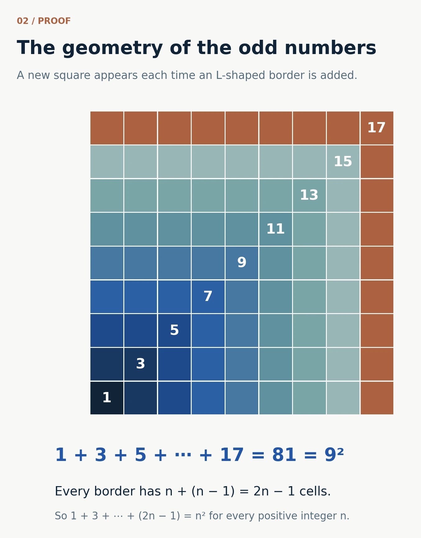
Tao’s concern about developing a proof involves something that a small diagram can make tangible. Knowing that the first n odd numbers add to n squared gives us a result. Figure 2 gives us a way to reconstruct it. Begin with the central cell and follow the coloured L-shaped borders outwards. Each enlarges the square by one cell along each side.

The outer border adds n cells along one edge and n − 1 along the other, making 2n − 1 new cells. That construction works for every positive integer and explains why the sum is a square. Someone who learns it gains an argument they can reconstruct and adapt. The research proofs released in October are vastly more complex, but extracting such reusable ideas from them is the work Tao wants the release to support.

Formal proof assistants add another way to check the logical chain. In Lean, a theorem is expressed in a precise language and its proof is checked by a small core program, the kernel. The guarantee concerns the formal statement, its definitions and the assumptions on which it depends. A reviewer still needs to establish that the formal statement captures the intended problem. Lean’s own validation guidance also explains why unfinished dependencies and additional axioms must be examined. A successful-looking build alone is an incomplete description of what has been verified. [2]

The OpenAI repository records different levels of verification. A result family can contain a principal argument, companion papers and alternative proofs, so manuscript totals count more than distinct solutions. The catalogue consulted on 10 October listed 719 manuscripts across 372 families and reported formalizations for approximately 42% of top-line results. Those figures describe that dated snapshot of an evolving repository. [4]

The Advisory Group on Mathematics and Artificial Intelligence, an independent group hosted at the Institute for Advanced Study in Princeton, has addressed how releases should support further mathematical work. Its September recommendations cover attribution, versioning, formalization status, access and community-led understanding. These are the conditions under which other researchers can examine a result, identify its dependencies and develop it. The group’s recommendations should be distinguished from a statement by the Institute as a whole. [5]

The potential reaches scientific computing through quite direct routes. AlphaTensor, reported by Alhussein Fawzi and colleagues in 2022, searched for matrix-multiplication algorithms and produced exactly checkable constructions, including improvements for particular finite-field settings. Matrix multiplication is a basic operation in simulation and machine learning. An improvement there can become useful far beyond the original mathematical problem, although a lower operation count in a specific setting does not automatically produce faster performance on every computer. [6]

An improved algorithm can reduce the cost of a calculation used in simulation or machine learning. A new theorem can also establish when an optimisation method converges or which measurements are sufficient to identify an unknown quantity. Following those consequences requires work beyond proving the initial result. In biology, a comparable change is already visible in the work that follows a predicted molecular structure.

Working from a protein structure

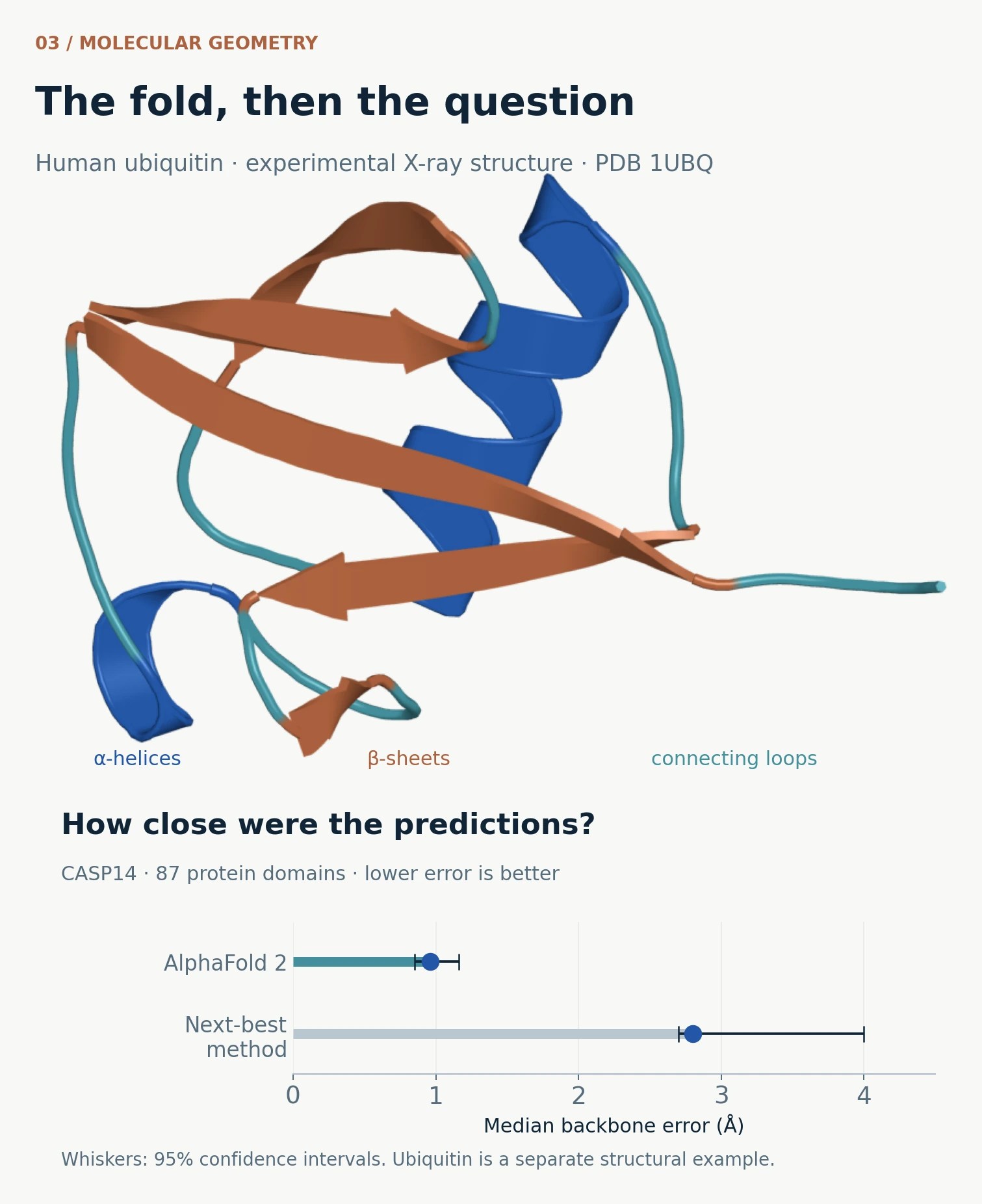
A biologist studying a protein needs to know how its amino-acid chain folds and which surfaces might contact other molecules. A three-dimensional structure makes those questions easier to investigate. Figure 3 shows human ubiquitin, a small protein whose experimental coordinates were deposited in the Protein Data Bank in 1987. Its folded shape contains spatial relationships that a sequence alone does not display. [7]

The two panels of Figure 3 connect the object being predicted to a measurement of prediction quality. Above is the experimental ubiquitin structure, showing what a folded protein looks like. Below is a separate benchmark across 87 protein domains from the 2021 AlphaFold paper by John Jumper and colleagues. AlphaFold’s median backbone error was 0.96 ångström, compared with 2.8 ångströms for the next-best method. An ångström is one ten-billionth of a metre; the smaller value means the predicted atom positions were closer to the experimental ones. The chart reports the benchmark, not a prediction of the ubiquitin shown above. [8]

That reduction in positional error made structural models more useful starting points for biological experiments. AlphaFold 3 extended predictions to complexes involving proteins, nucleic acids and small molecules. Its 2024 paper also reports clashes, stereochemical errors and incomplete treatment of alternative conformations. A predicted arrangement remains one view of a molecular system whose behaviour may involve many conformations in solution. [9]

A predicted arrangement of two cellular components can suggest how they interact and where an experiment might be informative. Their interaction in a cell also depends on when and where they are present, their abundance and competing partners. Researchers can use the structure to choose a focused measurement of that interaction, then revise their explanation in light of what they observe.

Having structural candidates early changes the order of that work. A group can compare possible explanations before committing to a difficult measurement, or use a model to investigate an unexpected observation. Places where predictions are uncertain may become useful targets for further experiments. The benefit then appears in the choice of experiment as well as the speed of producing a structure.

The ubiquitin coordinates also show how much this work depends on accumulated experimental records. The structure predates modern AI systems by decades. Public databases and the people who curate them make such measurements available to later researchers and model developers. Continued measurement supplies both the material for improving predictions and the independent evidence needed to assess them.

Learning from the next experiment

Once a structural prediction has suggested an experiment, the laboratory sets the pace. Samples have to be prepared and measurements collected. Chemistry offers examples of AI systems that participate in this stage too, choosing experiments and learning from their results.

In 2020, Benjamin Burger and colleagues reported a mobile robotic chemist that performed 688 experiments over eight days. A Bayesian search algorithm guided its exploration of a ten-variable space, and the search identified photocatalyst mixtures with six times the activity of the initial formulations. The robot carried out physical work in a laboratory; the measurements then guided subsequent choices. This is a specific demonstrated improvement in a defined experimental search, rather than evidence that every stage of chemistry had become autonomous. [10]

The robotic chemist had to choose where another experiment would be most useful. Figure 4 isolates one part of that decision in a calculated example. Compare the shaded band before and after the copper observation is added. The model samples where its uncertainty is greatest, and the new observation narrows the band nearby. A laboratory planner may make a similar choice when learning about an uncertain region is more valuable than retesting its current favourite.

The narrowing band shows what one additional observation contributes. Sometimes researchers can first narrow their candidates with calculations, reserving physical measurements for a smaller set. In the GNoME study, Amil Merchant and colleagues used learned models to screen crystal candidates, then assessed energetic stability with density-functional-theory calculations. They reported 381,000 new structures on an updated computed stability hull. Those were computationally assessed candidates for further investigation. [11]

Those calculations can narrow the set of materials worth making. A laboratory must still establish how to produce a sample, characterise it and measure its properties under useful conditions. For a battery material, a favourable energy estimate is one consideration among several demands on performance and manufacture. The screening result becomes valuable when it helps a group choose which candidates deserve that effort.

The record of each attempt matters to the next choice. A preparation failure and a reliably measured low-performing sample give different information. If the system treats both as an ordinary low score, it can learn the wrong relationship. More automated experiments increase the need to record what happened to the sample and whether the instrument produced a trustworthy measurement.

Predicting a changing atmosphere

Laboratory planners can usually choose when to take their next measurement. Weather forecasters work with an atmosphere that keeps changing as they calculate. Its sensitivity to initial conditions limits how far ahead a detailed prediction can remain useful. The Lorenz equations, introduced by meteorologist Edward Lorenz in 1963, make that sensitivity visible in a small mathematical system. [12]

In Figure 5, follow the two trajectories and then read the separation plotted beneath them. Both obey the same Lorenz equations, but their initial x values differ by one millionth. The lower plot shows that tiny difference becoming a large separation. This is why a forecaster needs to track uncertainty in the starting conditions, even with equations that describe the system precisely.

Forecasting systems seek better predictions over the period before such uncertainty overwhelms useful detail. GraphCast, described by Rémi Lam and colleagues in 2023, learned from historical atmospheric reanalysis and generated global forecasts up to ten days ahead. It outperformed its operational deterministic comparator on about 90% of 1,380 evaluated targets, each specifying a variable, level and forecast time. The Lorenz diagram explains the sensitivity that forecasting must contend with; these separate benchmark measurements establish GraphCast’s performance. [13]

Forecasting also benefits from describing possible futures and their probabilities. GenCast, published online in 2024 and in a 2025 issue of Nature, developed machine-learning ensemble forecasts and evaluated them against the European Centre for Medium-Range Weather Forecasts’ ensemble system. [14] An ensemble gives decision-makers something a single smooth prediction cannot: a view of how outcomes may vary. Its usefulness depends on whether the probabilities remain reliable when checked against events.

Physics and machine learning can also operate inside the same model. NeuralGCM, reported by Dmitrii Kochkov and colleagues in 2024, combines a numerical atmospheric dynamical core with learned components. Its work spans weather prediction and climate simulation. This approach preserves explicit physical structure while using learning for parts of the calculation that are difficult to represent adequately at the model’s resolution. [15]

A farmer choosing a planting date needs a forecast for a particular location and lead time. A city preparing for heavy rain needs useful information before it has to act. Evaluating those decisions calls for local performance measurements alongside global benchmarks. The cost of a missed event or a false alarm helps determine whether an improvement in prediction will be useful.

Choosing what to follow up

False alarms also matter when researchers screen molecules or materials. Useful candidates may be rare enough that a model’s shortlist still contains many failures, even after it has greatly improved the odds. The arithmetic determines how much laboratory work follows a prediction.

Figure 6 follows a screening decision from the full collection to the shortlist. Of 1,000 candidates, 20 are useful. A model that finds 80% of them selects 16 true leads; incorrectly selecting 5% of the other 980 adds 49 false leads. Follow the copper rings in the upper grid into the lower panel. Most selected candidates are false leads because the original collection contained so few useful ones. The numbers are a worked example of screening arithmetic.

The screen has increased the proportion of useful candidates more than twelvefold. It has also left 49 false leads to investigate. Whether that is a worthwhile exchange depends on the follow-up cost. A cheap calculation can tolerate a long shortlist more easily than an experiment that occupies an instrument for weeks. Scientific performance includes the work needed to find out which predictions succeed.

Researchers must also test what happens beyond the examples used to develop a model. A random split of closely related observations may exaggerate how well the system handles something unfamiliar. A stronger evaluation might hold out a later period, a different family of examples or a genuinely new experimental setting. The appropriate separation depends on the claim: future-weather performance, for example, poses a different test from interpolation within a previously studied dataset.

The ability to follow up a result also depends on access. A public manuscript can be examined even when the model that produced it is proprietary. Repeating the search may require access to that model, its data and its computing resources. In an automated laboratory, the apparatus adds another requirement. Researchers need to know which parts of a result they can reproduce and which they must take from the original group. [5]

The work after a result

The mathematicians responding to the October release were already facing this work. They had manuscripts to examine, students to advise and research programmes to reconsider. A proposed solution could contain an idea worth years of further study, but someone would have to find it, understand it and explain it well enough for others to use.

Biology and chemistry make the same demand through different kinds of evidence. A structural prediction becomes part of an explanation when researchers connect it to measurements of a living system. A screened material becomes a practical possibility when a laboratory can make and test it. Faster proposals allow more of these investigations to begin, while placing greater demands on the people and facilities that carry them through.

Funding and credit will influence which work gets done. Reading a difficult proof, curating experimental records or testing a failed prediction can require sustained expertise. If recognition attaches mainly to the first announcement, the work needed to develop its consequences may be left to researchers whose contribution is harder to see.

The next advance may emerge when a graduate student finds a reusable method inside an unfamiliar proof, or when an experiment reveals why a promising molecular prediction failed. Those are discoveries in their own right. Making room for them means giving researchers access to the tools, time to understand their outputs and credit for what they establish afterwards.

Sources and figure methods

Research checked: 10 October 2026. This feature draws on the original research papers, official proof-assistant documentation and the dated mathematical release below. The OpenAI collection is an evolving research repository; its figures describe the version consulted, not a final assessment of all its claims. The figures were created for 99Science from the cited coordinates, reported statistics, explicit calculations and explanatory diagrams. Download figure code and data.

1. Romera-Paredes, B. et al. (2023). Mathematical discoveries from program search with large language models. Nature 625, 468–475 (2024 issue). The FunSearch research paper.
2. Lean language reference. Validating a Lean Proof. Official documentation on formal statements, dependencies, axioms and levels of checking; accessed 10 October 2026.
3. OpenAI (6 October 2026). Sharing AI progress in mathematics. The release announcement and description of its supporting material.
4. OpenAI. Mathematics research repository, release history and formal proof artifacts. Catalogue and verification status checked 10 October 2026.
5. Advisory Group on Mathematics and Artificial Intelligence (29 September 2026). Responsible Release of AI-Generated Mathematics. Independent recommendations on attribution, verification, understanding and access.
6. Fawzi, A. et al. (2022). Discovering faster matrix multiplication algorithms with reinforcement learning. Nature 610, 47–53.
7. Vijay-Kumar, S., Bugg, C. E. & Cook, W. J. (1987). Structure of ubiquitin refined at 1.8 Å resolution. Journal of Molecular Biology 194, 531–544. Coordinates: PDB 1UBQ, chain A.
8. Jumper, J. et al. (2021). Highly accurate protein structure prediction with AlphaFold. Nature 596, 583–589. Figure 3 uses the reported CASP14 summary statistics; it does not reproduce a publisher figure.
9. Abramson, J. et al. (2024). Accurate structure prediction of biomolecular interactions with AlphaFold 3. Nature 630, 493–500. See especially the model-limitations discussion.
10. Burger, B. et al. (2020). A mobile robotic chemist. Nature 583, 237–241.
11. Merchant, A. et al. (2023). Scaling deep learning for materials discovery. Nature 624, 80–85.
12. Lorenz, E. N. (1963). Deterministic Nonperiodic Flow. Journal of the Atmospheric Sciences 20, 130–141. Figure 5 and the opening image are new numerical renderings of the model, not reproduced figures from the paper.
13. Lam, R. et al. (2023). Learning skillful medium-range global weather forecasting. Science 382, 1416–1421.
14. Price, I. et al. (2024, online; 2025, issue). Probabilistic weather forecasting with machine learning. Nature 637, 84–90.
15. Kochkov, D. et al. (2024). Neural general circulation models for weather and climate. Nature 632, 1060–1066.
16. SciPy reference. The Rosenbrock function. Definition of the optimisation test function rendered in Figure 1.

[17] Proofs and Prompts, 100+ reactions to 100+ solutions. Responses by Hugo Duminil-Copin and Terence Tao, published 8 October 2026. Their identities and awards are linked at first mention. Editorial revision checked 11 October 2026.